EXPLORING YOUR DATA

Introduction to Exploratory Data Analysis (EDA) using R

Dr. Ajay Kumar Koli | SARA Institute of Data Science

UGC - Malaviya Mission
Teacher Training Center
GJU of S&T, Hisar, Haryana

Download & Install


✅ R Software, https://cloud.r-project.org/

✅ RStudio IDE, https://posit.co/products/open-source/rstudio/?sid=1

✅ Quarto, https://quarto.org/docs/get-started/

RStudio


✅ Create RStudio Project in your computer

✅ Create quarto document

✅ Create folder data & save file penguins.csv

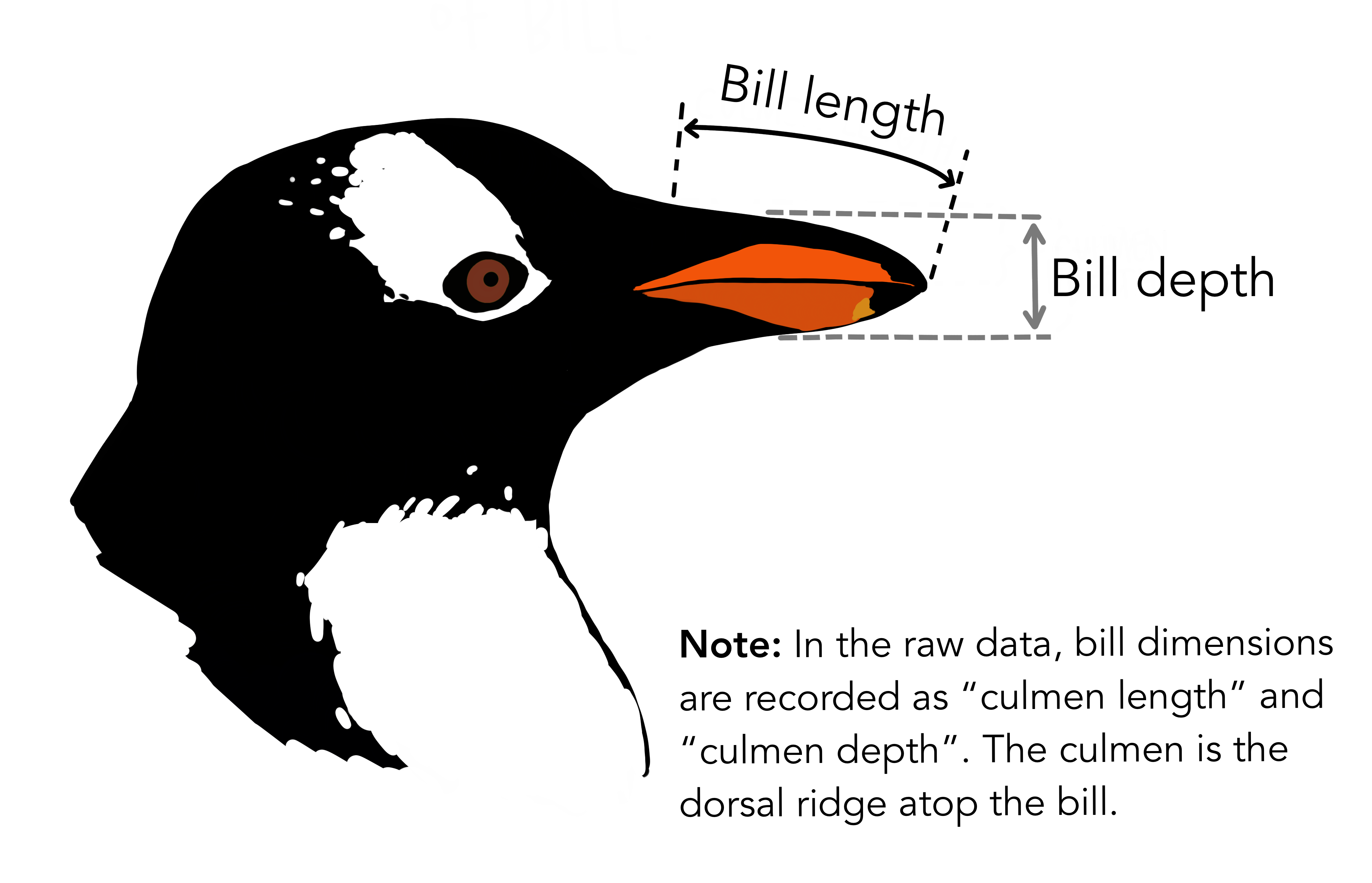
Data: penguins

Live on three island: Biscoe, Dream, & Torgersen.


Exploratory Data Analysis (EDA)


“how to use visualization and transformation to explore your data in a systematic way”

EDA using R:
10 Basic Steps

📦 Step 1: R Packages


Install R Packages only once:

```{r}
install.packages("palmerpenguins") # to get data
install.packages("tidyverse")      # to collection of R pkgs
install.packages("skimr")          # summary of data  
install.packages("janitor")        # data cleaning
```

Call/load R packages

```{r}
library(palmerpenguins)
library(tidyverse)
library(skimr)
library(janitor)
```

📁 Step 2: Import the Dataset

You can import from CSV, Excel, or other sources.


```{r}
library(readr)
penguins <- read_csv("session-1/practice/data/penguins.csv", 
    col_types = cols(sex = col_factor(levels = c("male", 
        "female"))))
View(penguins)
```
```{r}
# Replace with your actual file path
data <- read_csv("your_dataset.csv")   
```

Data Structure


📊 Step 3: Explore the Data Structure


```{r}
dim(data)          # Dimensions (rows & columns)

names(data)        # Column names

spec(data)         # columns specifications

head(data)         # First few rows

glimpse(data)      # Compact structure

str(data)          # Structure
```

Check Data for


  • Missing values

  • Duplicate rows

  • Inconsistent column names

✅ Step 4: Transform & Clean the Data

```{r}
library(readr)

penguins <- read_csv("data/penguins.csv", 
    col_types = cols(sex = col_factor(levels = c("male", "female")),
                     species = col_factor(levels = c("Chinstrap",
                                                     "Gentoo",
                                                     "Adelie")),
                     island  = col_factor(levels = c("Biscoe",
                                                     "Dream",
                                                     "Torgersen"))
                     ))
```


```{r}
summary(penguins)         #basic summary
```
```{r}
sum(is.na(penguins))                 # Total missing values
colSums(is.na(penguins))             # Total column wise missing values       
```

Variation

  • “It is the tendency of the values of a variable to change from measurement to measurement or across different subjects or at different times.”

  • “Every variable has its own pattern of variation, which can reveal interesting information about how it varies between measurements on the same observation as well as across observations.”

Variation Types

  1. What type of variation occurs within my variables?

  2. What type of co-variation occurs between my variables?

📈 Step 5: Univariate Analysis

Explore each variable individually

```{r}
summary(data$variable)
hist(data$variable, main="Mass Distribution", col="lightblue")
```

Use ggplot2 for more control

```{r}
ggplot(penguins, aes(x = body_mass_g)) +
  geom_histogram(fill = "skyblue", bins = 30, color = "white") +
  labs(title = "Distribution of Body Mass (g)", x = "Body Mass (g)") +
  theme_minimal()
```
```{r}
table(data$variable)
barplot(table(data$variable), col="pink", main="Species Count")
```

Use ggplot2 for more control

```{r}
ggplot(penguins, aes(x = species)) +
  geom_bar(fill = "steelblue") +
  labs(title = "Penguin Species Count") +
  theme_minimal()
```

🔁 Step 6: Bivariate Analysis

Explore relationships between variables

```{r}
ggplot(penguins, aes(x = flipper_length_mm, y = body_mass_g)) +
  geom_point(aes(color = species)) +
  geom_smooth(method = "lm", se = FALSE) +
  labs(title = "Flipper Length vs Body Mass") +
  theme_minimal()
```
```{r}
ggplot(penguins, aes(x = species, y = body_mass_g, fill = species)) +
  geom_boxplot() +
  labs(title = "Body Mass by Species") +
  theme_minimal()
```

📌 Step 7: Summary Statistics


```{r}
skimr::skim(data)         # Rich summary
```

📉 Step 8: Outlier Detection

An outlier is a data point that differs markedly from the rest of the data.


```{r}
ggplot(penguins, aes(y = body_mass_g, x = species, fill = species)) +
  geom_boxplot() +
  labs(title = "Outliers in Body Mass by Species") +
  theme_minimal()
```

🧹 Step 9: Handle Missing Data


(if needed)

```{r}
# Fill missing values
penguins$body_mass_g[is.na(penguins$body_mass_g)] <- median(penguins$body_mass_g, na.rm = TRUE)

summary(penguins$body_mass_g)
```
```{r}
# Remove rows with missing data
penguins_clean <- penguins %>% drop_na()
dim(penguins_clean)
```

🧾 Step 10: Save Cleaned Data


```{r}
write.csv(data_clean, "cleaned_data.csv")
```

🎯 Learnings

  1. Installing R, RStudio, Quarto & R packages.
  2. Import & export of Data
  3. View summary & structure of data
  4. Table & plots to see pattern in data
  5. Treating missing & outlier values


Savitribai Ramabai (SARA) Institute of Data Science


Contact SARA


925 315 2024

sara.institute.info@gmail.com

www.sara-edu.netlify.app/

SARA Institute of Data Science,
Dr. Ambedkar Bhawan, Kakroi Road, Near Dayanand Hospital,
Sonipat - 131001, Haryana, India.


Thank-You!